Reznick (2007) (see previous post) simplified Robinson simplification of Hilbert construction of positive polynomials that are not sums of squares by his perturbation lemma. Blekherman shows that the mystery is in the dimension of monomial basis. For example, there are  points in n-dimensional hypercube, but since there are only
  quadratic monomials all this points when evaluated cannot have rank more then the number of monomials. As a consequence, it is sufficient to nullify only about quaratic number of points in a quadratic form (by applying a set of linear constraints on the coefficients arising from evaluations of values of monomials) to nullify all points in a hypercube for these quadratic forms.
There are much more monomials in quartic polynomials (much larger basis), and therefore much larger freedom in choosing coefficients such that quartic will be nullified at quadratic number of points in hypercube, but will be nonzero on other points of a hypercube! That lead that such quartic polynomial even if it will be positive will not be a sum of squares.
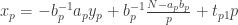
Reznick perturbation lemma open a way to automatically (algorithmically) generate positive polynomials that a re not sums of squares, which in the current version may not lead to sufficient expansion of positive polynomial cone to solve all the problems from a given class. Reznick (2007) perturbation lemma, simplified for our current purpose, in high school terms, starts from a sums of squares of terms defining hypercube, say  is
is 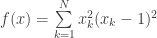 . Moreover, at the minimum it round, i.e. Hessian is strictly positive definite (easy to check by direct calculations, intuitively each term in the sum around the minimum is a positive definite quadratic multiplied by approximately 1). Now we are going to perturb this quartic by another quartic (
 ), splitting points in the hypercube into two sets. In one set we require that Taylor expansion of vanish to second order term, and on the other set we require that is strictly positive. Only those points in the hypercube are dangerous, since perturbation
  may lead to negative values around minima for any positive
  . In the rest of the space we can choose small enough to ensure positiveness of resulting polynomial (I skip this part, but one need to have worst estimate for the values of for a given norm of
  and take a region bounded by some norm and outer region where only ratios between leading coefficients matter). For the first set of points has Hessians with the finite eigenvalues. If we need to ensure that c times minimum eigenvalue is smaller that Hessian eigenvalues (all the same) for
  in the minima. That ensures 0 value on the set that are local minima. For the second set of points the value is positive in some neighborhood by construction.
Now automatic construction: given monomial basis we need to ensure about quadratic number of points to have 0 values and gradients being 0. That is about  conditions for about
  monomials. The rest of points in the hypercube should be strictly greater than zero. For that we need to ensure that the values at the basis points are positive and that all point in the hypercube are represented by the linear combinations with positive coefficients. For that we need to peak as the basis points the points with minimum number of ‘1’ as coordinates. and the second condition is the inequality condition. leading to linear program. It has solution because we have coefficients in front of
  that can grow unbound, and being compensated by other terms. and inequality condition is much weaker then equality condition. Then one can compute the estimate for the constant c, which depends only on the calculations in the basis points. The exact machinery still need to be worked out, since one need also estimate the values of projections of all point of hypercube onto basis points.
That may be not sufficient to produce wide enough expansion of SOS cone to solve all instances of, say, partition problem, but we may need small enough extension to pertube problem quartic to be represented by the sums of squares.
Sincerely yours,
C.T.
PS
psd that is not SOS:

and the (not cleaned) code in Matlab with symbolic toolbox to get it
%% mupad test for positive polynomials Hilber-Reznik

n=3;
y= evalin( symengine, sprintf( 'combinat::compositions(4, Length= %d, MinPart=0)', n+1) );
pow= arrayfun( @(k) double(y(k)), 1:numel(y), 'UniformOutput', false );
pow= cat(1, pow{:});
xs= sym( 'x', [n,1]);
xx= zeros( 2^n, n );
v=0:2^n-1;
for k=1:n,
xx( bitand(v, 2^(k-1) )~=0 , k )=1;
end
%xx= 2*xx-1;
xx(:, n+1)=1;
%xx( end+1, :)= [1 2 2 1];
y= evalin( symengine, sprintf( 'combinat::compositions(2, Length= %d, MinPart=0)', n+1) );
pow2= arrayfun( @(k) double(y(k)), 1:numel(y), 'UniformOutput', false );
pow2= cat(1, pow2{:});
yy2= nan( size( pow2,1), size(xx,2) );
yy= nan( size( pow,1), size(xx,2) );
for k=1:size(xx,1),
yy(:, k)= prod( bsxfun( @power, xx(k,:), pow ), 2);
yy2(:, k)= prod( bsxfun( @power, xx(k,:), pow2 ), 2);
end
for k=size( pow, 1 ):-1:1,
xsm( k )= sym(1);
for k2= n:-1:1,
xsm( k )= xsm( k )*xs(k2)^pow( k, k2 );
end
end
for k= n:-1:1,
dxsm(k,:)= diff( xsm, xs(k) );
end
r= rank(yy2);
x0Idx= 1:7;
x1Idx= 8;
%we need also condition for gradient here
dpow= zeros(size(pow));
dpow(:,end)=1;
for k=1: size( pow, 2)-1,
idx= pow(:,k)>0;
dpow( idx, end )= dpow(idx, end).*pow(idx,k);
dpow(idx,k)= pow(idx,k)-1;
end
% %
% equality constraints
lc= zeros(size(pow, 1), 0);
for k=1:7,
lc(:, end+1)= subs( xsm, xs, xx(k, 1:3) )';
lc(:, end+(1:n))= subs( dxsm, xs, xx(k, 1:3) )';
end
% lc(:, end+(1:n))= subs( dxsm, xs, xx(8, 1:3) )';
%%%%%%%%%%%%%%%%%%%%%%%%%%%%%%%%%%%%%%%%%%%%%%%%%%%%%%%%%%%%%%%%%%%%%%%%
%
% The following line is a place to play with different polynomials
% we have rather strange way to do it here by imposing eight point
% where quartic polynomial vanishes first order term on Taylor expansion,
% and the value at this point is positive (it is sufficient to have 0 here,
% but the code would be more complicated).
% removing second line below (lc .. ) and switching next lc lines
% (commenting/ uncomenting) lead to Robinson polynomial
%
%%%%%%%%%%%%%%%%%%%%%%%%%%%%%%%%%%%%%%%%%%%%%%%%%%%%%%%%%%%%%%%%%%%%%%%%%
x2= [3 -3 3]; % [3 -1 3] also works well
lc(:, end+(1:n))= subs( dxsm, xs, x2 )'; % comment for Robinson
bc= zeros( size( lc, 2), 1 );
% lc(:, end+1)= subs( xsm, xs, xx(8, 1:3) )'; % uncomment for Robinson
lc(:, end+1)= subs( xsm, xs, x2 )'; % comment for Robinson
bc(end+1)=1;
%%%%%%%%%%%%%%%%%%%%%%%%%%%%%%%%%%%%%%%%%%%%%%%%%%%%%%%%%%%%%%%%%%%%%%%%%%%%%%%%%%%
cf= mldivide( lc', bc)*54*2 % multiplier 1 for Robinson
disp( [size(lc) rank(lc)])
% %
% coefficient c in perturbation lemma was found by hand, and in now way is optimal
p2= 1/1000*sum( round(cf).*xsm.') + sum( xs.^2.*(xs-1).^2) % first factor is 1 for Robinson
dp2= [diff(p2, xs(1)) diff(p2, xs(2)) diff(p2, xs(3))]
subs( p2, xs, xx(8, 1:3))
sol= solve(dp2)
xv= ([sol.x1 sol.x2 sol.x3]);
vf= arrayfun( @(k) double(subs( p2, xs, xv(k, :))), 1:size(xv,1))';
[min(vf) min(real(vf)) min(imag(vf))]


 is it possible to divide it into complementary multisets having the same sum, i.e. whether there exist
  such that
  .
. each, decide whether all clauses can be satisfied (evaluated true) at once. To encode it, we want the set of polynomial equation evaluating 0 when clause is true:
  would be translated into
  .
. ,
, ,
, ; for 3-SAT:
  , where
  is one 3 term clause. The last equation is not always positive, but for large enough
  it is, when problem is not satisfiable, thanks to third ingredient.
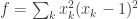 ), condition 1 in the Lemma. If NP-complete problem is not satisfiable
  , condition 2. Finally,
  , where
  are zero set of
  , a set of
  that
that  is positive.
 . This is
  , i.e. we replace
  , we say negation (by analogy with binary variables and there translation to polynomials). This is also extremal positive polynimial that controls value at (0,1,1). Same way we can make all extremal polynomials that controls independently all vertices of a hypercube. Let
  be a linear combination of all Robinson polynomials controlling different vertices of hypercube in 3 variables with positive coefficients (i.e. a point inside the cone of positive polynomials defined by the Robinson polynomials).Now consider polynomial
  . Once the value of this polynomial at
  is positive, there exists
  such that this polynomial is positive! The same is true if we sum up all negations of quartic:
 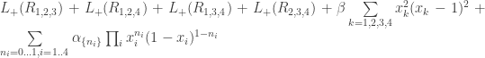 . Once values on 16 hypercube vertices are positive there is
  that for all
  the polynomial is positive. Note that all 16 vertices are controlled independently.
 for 3-SAT and
  for partition problem. It adds additional freedom in the choice of variables, and limits the value of
  being quite small.
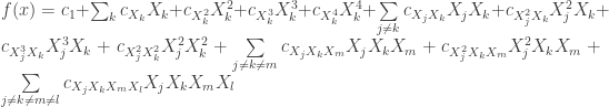
 which have clear solution, we can now peak a cubic point around solution (very close) and require the qurtic polynomial to be round at this points (i.e. the value and gradient are zero at these points and Hessian is positive definite ) than this polinomial will be positive and is not sum of squares. More generaly, the quartic polynomial will positive if more than square points (number of monomials in quadratic polinomial of the same dimension) are round and there is continuous path to original sum of squares such that this property holds for every point in the path. That would an alternative ( to Hilbert method) way to construct positive polynomials.
 , where
  and
and  are some polynomials it is obvious that
  , where
  is an arbitrary unique symbol denoting variable. For example,
  . Let
. Let  being evaluation of the set
  at point
  for any point x,
  .
.  , where
  . Let polynomial be a linear combination of elements of
  , where
  enumerates elements of the set.
 . Integer partition problem is asking whether
  , e.g. whether it is possible to divide set of integers into two complementary sets that have equal sum. This problem is NP-complete.
 is greater than zero or not.
 . The second sum at given values can be zero only when partition exists
 than
than  .
.
 .
. .
. , taking into account second case.
 , which is clearly 0 for
  , since in each term in the sum either first or second factor is 0
 .
. .
. , taking into account second case.
 , since we are interested in positive polynomials. Necessary condition is that gradient equals 0 for corresponding points.
 .
. .
. is splitted into 2 cases.
  and
and 
 together with
  that lead to
 .
. split again into the same cases.
 together with
  and
and  that lead to
  .
. . The last condition counted over triplet lead to Robinson perturbation term

 zeros forming n-simplex than its form is constrained. After a linear transformation this simplex can be transformed into standard orthogonal simplex with zeros being at
 . Zero gradient (necessary for quartic being positive) leads to
  . Zeros at other vertices lead to the following constraint
  , whereas zero gradient leads to
 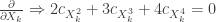 leading to null-space
  , i.e.
  for any
  , where
  coefficients in quadratics. For the corresponding quartic we need at least
  generic points where quartic and its gradient vanish. That leads to
  constraints. We need more coefficients to have some freedom. That is achievable for the dimension more than 5. That is saying that perturbation can be very strong.
 with
with  entries tell whether it is possible to divide it into two miltisets having the same sum. Formally, tell whether there exists vector
  such that
  , or in vector notation
  . This problem is NP-complete.
 , where
  is positive semidefinite polynomial ( a polynomial that is non-negative over whole range of values
 ![a= [1, 1, 1, 1, 1]](https://s0.wp.com/latex.php?latex=a%3D+%5B1%2C+1%2C+1%2C+1%2C+1%5D+&bg=ffffff&fg=333333&s=0&c=20201002) is strictly positive. Here we need to generate enough PSD that certainly have no solution. Then we would have a complete basis for PSD polynomials and solve the problem, which would be an instance of linear programming in this case (details for similar problem can be found in
is strictly positive. Here we need to generate enough PSD that certainly have no solution. Then we would have a complete basis for PSD polynomials and solve the problem, which would be an instance of linear programming in this case (details for similar problem can be found in  runners having distinct constant speeds
  start at a common point (origin) and run laps on a circular track with circumference 1. Then, there is a time when no runner is closer than
  from the origin.
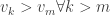 .
. is the number of whole laps (including 0) runner k passed on a track, than
  and
and  .
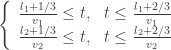
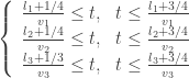
. runner 1 is exactly distance
  (
( ).
).
 we can eliminate it if all combination of left parts on the left columns are smaller than any right parts in the right column of the table. e.g.


 and
and  satisfying inequality
 lead to (remeber that
  )
)


 since
since  In other words,
  satisfying inequality.
 in terms of
 satisfying initial inequalities and LRC holds.
 inequalities
 in terms of
  and
and  in terms of
  and
and 


 if
if 
 is tight distance.
 start at a common point (origin) and run laps on a circular track with circumference 1. Then, there is a time when no runner is closer than
  runners is discussed
  .
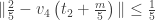
.  denote the distance of x to the nearest integer.
 . At time
  all runners are at least
  from the origin. Done.
 . There is time
  such that runners
  are at least
  from the origin – see case
  . At time
  runners
  are at the same positions as runners
  at time
  ,
,  we are done. Otherwise, since
  and 5 are co-prime,

 . Done.
 .
. .
. are at least
  from the origin – see case
  . Since
  and 5 are co-prime those runners visit all sectors once at times
  , and runners 1 and 2 will be at the same position. There 5 such times, during 2 times runner 3 will be at sectors
  and during 2 times runner 4 will visit the same sectors. Therefore, there is
  . Done.
 .
. . If there more than one way choose the one with maximum sum. We have 2 sub-cases:
  ,
,  .
. . The runner 1 is faster than either runner 2 or 3. Therefore, they meet at distance greater than
  this runner is slower than either runner 2 or 3 (call this runner
  ) which is at the same position as runner 4. Therefore, it will meet runner 1 later than runner
  . This runner should move fast to reach runner 1 at distance
  of the lap. Then, looking at opposite direction in time in the same time it will cover the same distance, and will be at least
  from the origin when runner 1 reach distance
  . Done.
 runners 2 and 3 are the same distance from the origin on the opposite sides from the origin.
  . It makes
  cycles, where
  stands for
  . If
. If  half of the time runner 1 is away from the origin. With larger
  there is bigger fraction, with the limit
  . Let
. Let  is the time when runner 1 is distant. At the same time runners 2 and 3 same distance on the opposite sides from the origin. Now at times
  runner 1 stays at the same position, runners 2 and 3 are on the opposite position relative to the origin, and runner 4 visiting all sectors once each time. Therefore, there are total 2 moments when runner 4 in
  . Done.

 and
and  bring new ingredients (non prime
  .
.  . where the infimum is taken over all n-tuples
  of distinct positive integers.
 the LRC state that
 .
.  are relatively prime. At time
  two runners are at the same distance from the origin from different sides of the lap at distances proportional to
  . Since they are relatively prime both runners visit all the points
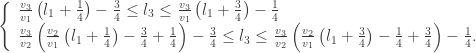
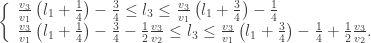
  . The largest distance is
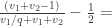
 ![\frac{ \left[ \frac{v_1+v_2}{2} \right] }{v_1+v_2}](https://s0.wp.com/latex.php?latex=%5Cfrac%7B+%5Cleft%5B+%5Cfrac%7Bv_1%2Bv_2%7D%7B2%7D+%5Cright%5D+%7D%7Bv_1%2Bv_2%7D&bg=ffffff&fg=333333&s=0&c=20201002) , where
, where ![\left[ \circ \right]](https://s0.wp.com/latex.php?latex=%5Cleft%5B+%5Ccirc+%5Cright%5D&bg=ffffff&fg=333333&s=0&c=20201002) means integer part.
means integer part.  , at times
  runners are at positions
  and
and  and the maximum distance from origin is
 ![\frac{\left[ \frac{1+2}{2}\right]}{3}= \frac{\left[1.5 \right]}{3}= \frac{1}{3}](https://s0.wp.com/latex.php?latex=%5Cfrac%7B%5Cleft%5B+%5Cfrac%7B1%2B2%7D%7B2%7D%5Cright%5D%7D%7B3%7D%3D+%5Cfrac%7B%5Cleft%5B1.5+%5Cright%5D%7D%7B3%7D%3D+%5Cfrac%7B1%7D%7B3%7D&bg=ffffff&fg=333333&s=0&c=20201002) .
.  , the maximum distance is
  .
.  the maximum distance is
  at time
  with the minimum for runners at speeds
  . Therefore,
  .
.  , e.g
, e.g  .
.
 runner 3 is at the origin. There is a time such that some time before it was the same distance with runner 1 and some time after it will be the same distance with runner 2. (The situation is reversed at times
  ). We are interested when that is happening for the time runners 1 and 2 are most distant from the origin.
  with speed
  , so the time needed is
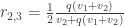
  . Runner 3 passes
 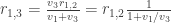 . Therefore, the closest point is reached when
  is maximum.
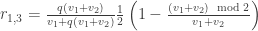
 ,
,  around
 .
.


 .
. 

![\frac{2 v_1+ 2 v_2 - 2 - v_1/q - v_1-v_2 }{2 \left[ v_1/ q+ ( v_1+v_2 ) \right] } =](https://s0.wp.com/latex.php?latex=%5Cfrac%7B2+v_1%2B+2+v_2+-+2+-+v_1%2Fq+-+v_1-v_2+%7D%7B2+%5Cleft%5B+v_1%2F+q%2B+%28+v_1%2Bv_2+%29+%5Cright%5D+%7D+%3D+&bg=ffffff&fg=333333&s=0&c=20201002)
![\frac{ v_1 \left( 1- \frac{1}{q} \right)+ v_2 - 2 }{2 \left[ v_1/ q+ ( v_1+v_2 ) \right] }](https://s0.wp.com/latex.php?latex=%5Cfrac%7B+v_1+%5Cleft%28+1-+%5Cfrac%7B1%7D%7Bq%7D+%5Cright%29%2B+v_2+-+2+%7D%7B2+%5Cleft%5B+v_1%2F+q%2B+%28+v_1%2Bv_2+%29+%5Cright%5D+%7D+&bg=ffffff&fg=333333&s=0&c=20201002) . Since
. Since  nominator is greater than 0, except when
 .
. only for
  .
. .
.
 . Let
. Let  be the distance from the origin of runner 3 at the moment
  be the distance of the runners 1 and 2 from the origin at the same time. The maximal distance when runners 1 and 2 or 1 and 3 equidistant around time
  .
. be the speed of the runner 1 or runner 2 moving in opposite direction, so that the difference in distances is decreasing moving either forward or backward in time. Since
  runner 3 will cover greater distance away from the origin that other runner
  , and
, and  – distance of runner 3 from the origin.
  .
. ,
, 
 .
. only for runners
  , where index
  enumerates rows, and index
  enumerates columns. Each element
  and
and  . Suppose
  is a realization of random variables. We are going to fix it for the rest of the post.
  . Since,
  ) where the first column has value
  :
:  . Since
  with probability one. Moreover, viewing
  , and
, and  is a realization of equi-probable binary random variable.
 such that
  . We select from the table
  . The set
  consists of countable infinite number of rows with probability 1. Moreover, the table
  – all rows coincide with
  . The right part – all columns starting from
  are realization of independent random variable.
 that is countably infinite with probability 1, and each member consists of rows
  than we have countable infinite representation of power set of countably infinite set by the theorem, whereas Cantor diagonal argument says the opposite. Therefore, if one replace the axiom of choice with the axiom of “free will’ – there exist Bernoulli process one have contradictory statement about sets cardinality. Axiom of choice is than deductible from the fact that all members of the sets
  shows there are countable many reals, and moreover there are countable many equal reals.
 and equations
  , one can expact 64 dimensional nullspace in the space of monomials of some degree. The above show that in the usual Nullstellensatz case one need 8th order monomials, whereas it is sufficient to have tautologies variables of equivalent degree 6. This is on decoding side.
 . In tautology variables it is linear equation, but than one can split it into two halves on the right and left side and square it. One can also take cubes, that is still possible since we are looking at equivalent 6th order polynomials. One has exponentially many ways to split encoding equation. The question here how to extract relevant information in, say, polynomial time.
